Calculating the gluPerspective matrix and other OpenGL matrix maths

All 3D graphics programming requires that we manipulate matrices, for transformation and projection. Since graphics toolkits give us the matrix formulae directly, it is very easy to go on using them without truly understanding how they work. When we use OpenGL, the first thing we are told is to “just call” a bunch of matrix manipulation functions, like glTranslate, glScale, gluPerspective, etc, and it’s easy to go on building 3D worlds without understanding how these matrices work. But I like a deep understanding of how my software works, so I wanted to work out the maths behind these matrices. In particular, as we move towards OpenGL 3.0 and 4.0 and OpenGL ES 2.0, these newer standards are removing all of the built-in matrix stuff (for example, all of the above three functions have been removed) and you have to do all of this stuff manually.

I haven’t been able to find a good analysis of how to derive the matrices. In particular, the perspective projection matrix has often baffled me. So, I worked it all out and this post is a complete working of how to calculate several transformation and projection matrices, including perspective projection. This post is very heavy on mathematics, but I’ll try not to assume much, and if you already understand the basics of matrix transformations, you can just skip ahead.

The OpenGL coordinate system

This section covers the basics of coordinates, vectors and the OpenGL transformation pipeline. You can skip ahead if you already know this stuff.

In OpenGL, each vertex is represented by a point in 3-dimensional space, given the coordinate triple (x, y, z). Traditionally, you would specify a vertex using glVertex3d (or, in 2D graphics, with glVertex2d, which sets z to 0). Unfortunately, it’s quite confusing what the three axes actually mean in 3D space, and it is more confusing because a) it tends to be different from one platform to another (e.g., DirectX uses a different coordinate system to OpenGL which uses a different one to Blender, for example), and b) it can change based on how you set things up (e.g., by rotating the camera, you can change which direction is “up”). So for now, let us assume the default OpenGL camera and we’ll discuss how to transform the camera later.

OpenGL uses a right-handed coordinate system by default, meaning that if you hold out your right hand, extending your thumb, index and middle fingers so that they form three perpendicular axes (as shown in the image below), your thumb shows the direction of the positive X axis, your index finger the positive Y axis, and your middle finger the positive Z axis. Clearly, once your fingers are in place, you can orient your hand any way you like; the default OpenGL orientation is that X extends to the right, Y extends upwards, and Z extends towards the camera.

The right-handed coordinate system used by OpenGL

What I find strange about the OpenGL coordinate system is the orientation of Z. Since the positive Z axis runs towards the camera, it means that every visible object in the scene needs to have a negative z coordinate, which seems a bit un-intuitive. I would find a left-handed coordinate system (where Z extends away from the camera) to be more intuitive. You can use the camera or projection matrices to obtain a left-handed coordinate system, but it is probably simpler to stick to the defaults to avoid confusion.

The unit of measurement in OpenGL is “whatever you like”. In 2D graphics, we are used to measuring things in pixels, but in 3D graphics, that doesn’t make sense since the size of something in pixels depends upon how far away it is. So OpenGL lets you use arbitrary “units” for describing sizes and positions. One good thing about this, even for 2D graphics, is that it makes the display resolution independent — adjusting the screen resolution won’t alter the size of objects on the screen, it will simply adjust the level of detail.

What OpenGL is really about, at its core, is working out how a bunch of vertices go from floating around in 3D space and end up on your screen (a 2D space). The fact that vertices are used to connect polygons together is largely irrelevant (most of the hard work is in transforming vertices; once they are transformed, the polygons can be rendered in 2D). There are several considerations here:

• Artists and programmers do not like defining every single vertex in its final position in 3D space. That would be crazy, because then whenever an object moved, we would have to adjust all of the vertices. Rather, we want to define every vertex relative to the centre of the particular model (such as a car or person), and then transform the whole model into its position in the world.
• We need to be able to move the camera freely around the world. To do that, we need to be able to transform all of the vertices in the entire world based on the position and orientation of the camera. (You can think of the camera in OpenGL as being stationary at point (0, 0, 0) facing the -Z axis; rather than moving the camera, we must translate and rotate the entire world into position relative to that fixed camera.)
• The screen is a 2D surface. Rendering a 3D image onto a 2D surface typically requires some sort of perspective, to make objects that are further away seem smaller, and objects that are closer seem larger. Also, 2D screens are usually not square, so in transforming to a 2D display, we must take into account the aspect ratio of the screen (the ratio of the width and height). On screens with a wider aspect ratio (such as widescreen 16:9 displays), we need to show more objects to the left and right than on screens with thinner aspect ratio (such as full screen 4:3 displays).
• The screen is made up of pixels, and so when we render the display, we need to know each vertex’s position in pixels (not arbitrary OpenGL units). So we must transform the arbitrary units into pixels so that our scene fills up the whole screen at whatever resolution the display is using.

These considerations roughly form a series of steps that each vertex must go through in its journey from 3D model space to the screen. We call this the vertex pipeline, and OpenGL takes care of most of it automatically (with a little help from the programmer). Newer versions of OpenGL force the programmer to program much of the pipeline his/herself. To describe the pipeline, we must come up with a name for the “coordinate space” at each step of the way. These are outlined in the official OpenGL FAQ:

• Object Coordinates are the coordinates of the object relative to the centre of the model (e.g., the coordinates passed to glVertex). The Model transformation is applied to each vertex in a particular object or model to transform it into World Coordinates.
• World Coordinates are the coordinates of the object relative to the world origin. The View transformation is applied to each vertex in the world to transform it into Eye Coordinates. (Note: In OpenGL, the Model and View transformations are combined into the single matrix GL_MODELVIEW, so OpenGL itself doesn’t have a concept of world coordinates — vertices go straight from Object to Eye coordinates.)
• Eye Coordinates are the coordinates of the object relative to the camera. The Projection transform is applied to each vertex in the world to transform it into Clip Coordinates. (Note: In OpenGL, the Projection transformation is handled by the GL_PROJECTION matrix.)
• Clip Coordinates are a weird intermediate step which we will discuss in detail later. They are transformed by the Divide step into Normalised Device Coordinates, which I will abbreviate as Viewport coordinates.
• Viewport Coordinates (or Normalised Device Coordinates in the OpenGL specification) are the coordinates of the vertex in their final on-screen position. The x and y coordinates are relative to the screen, where (-1, -1) is the lower-left corner of the screen and (1, 1) is the upper-right corner of the screen. The z coordinate is still relevant at this point because it will be used to test and update the depth buffer (briefly discussed in the next section); a z of -1 is the nearest point in the depth buffer, whereas 1 is the furthest point. (Yes, this really confuses me too: the Z axis flips around at this point such that the +Z axis extends away from the camera, while the -Z axis points towards the camera!) Any vertex outside the cube (-1, -1, -1) to (1, 1, 1) is clipped, meaning it will not be seen on the screen. The Viewport transformation is applied to the (x, y) part of each vertex to transform it into Screen Coordinates.
• Screen Coordinates are the (x, y) coordinates of the vertex in screen pixels. By default, (0, 0) represents the lower-left of the screen, while (w, h) represents the upper-right of the screen, where w and h is the screen resolution in pixels.

In the “old” (pre-shader) OpenGL versions (OpenGL 1.0 and 2.0 or OpenGL ES 1.1), you would control the Object to Eye coordinate transformation by specifying the GL_MODELVIEW matrix (typically using a combination of glTranslate, glScale and glRotate), and the Eye to Clip coordinate transformation by specifying the GL_PROJECTION matrix (typically using glOrtho or gluPerspective). In the “new” (mandatory shader) OpenGL versions (OpenGL 3.0 onwards or OpenGL ES 2.0 onwards), you write a shader to do whatever you want, and it outputs Clip coordinates, typically using the same model, view and projection matrices as the old system. In both systems, you can control the Viewport to Screen transformation using glViewport (but the default value is usually fine); everything else is automatically taken care of by OpenGL. In this article, we are most interested in the transformation from Object coordinates to Viewport coordinates.

The depth buffer

I very briefly digress to introduce the OpenGL depth buffer. You can skip ahead if you already know this stuff.

While OpenGL draws pretty colourful objects to our screens, what is less obvious is that it is also drawing the same objects to a less glamorous greyscale off-screen buffer known as the depth buffer. When it draws to the depth buffer, it doesn’t use pretty lighting and texturing, but instead sets the “colour” of each pixel to the corresponding z coordinate at that position. For example, I have rendered the Utah teapot (glutSolidTeapot), and the images below show the resulting colour buffer (the normal screen display) and the depth buffer. Notice that the depth buffer uses darker pixels for the parts of the teapot that are closer to the screen (such as the spout), while the parts further away (such as the handle) fade off into the white background.

The colour buffer

The depth buffer

The closest physical analogy I can think of is if you imagine you are in a room where all objects are completely black, but there is a very thick white fog. In this room, the further away something is, the lighter it appears because there is more fog in between your eye and the object. If you have ever seen an autostereogram, such as Magic Eye, they often print “answers” in the form of a depth map (such as this shark), and these are essentially the depth buffer from a 3D scene.

The depth buffer has several uses. The most obvious is that every time OpenGL draws a pixel, it first checks the depth buffer to see if there is already something closer (darker) than the pixel it is about to draw. If there is, it doesn’t draw the pixel. That is why you usually don’t have to worry about the order you draw objects in OpenGL, because it automatically avoids drawing a polygon over the top of any polygon that is already closer to the screen. If you didn’t have the depth buffer, you would have to carefully draw each object in order from back to front! (That is why you need to remember to call glEnable(GL_DEPTH_TEST) in any 3D program, because the depth buffer is turned off by default!)

It is important to note that the depth buffer does have a finite range, which is implementation-specific. Each depth buffer pixel may, for example, be a 16-bit integer or a 32-bit float. The z values are mapped on to the depth buffer space by the projection matrix. This is why, when you call gluPerspective, the choice of the zNear and zFar values is so important: they control the depth buffer range. In the above image, I set zNear to 1 and zFar to 5, with the teapot filling up most of that space. Had I set zFar to 1000, I could see a lot further back, but I would be limiting the precision of the depth test because the depth values need to be shared over a much wider z space.

Simple matrix transformations

This section covers the mathematics of the scale and translate matrices. You can skip ahead if you already know this stuff.

Let’s say we want to apply a scale transformation of (100, 30, 10) to an object. Mathematically, this is very simple: just take each of its vertices and multiply the x value by 100, the y value by 30, and the z value by 10, like this:

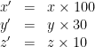
To do this efficiently, we can express the transformation as a matrix. Modern graphics cards can do matrix multiplication extremely quickly, so we take advantage of this wherever possible. We can express the scale as a 3×3 matrix:

If we express a vector as a 1×3 matrix:

Then we can apply the scale simply by multiplying the scale matrix by the vector:

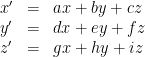
See the Wikipedia article Matrix multiplication for an explanation of how this works. In general, we can think of a matrix as a function that transforms a vector in a very restrictive way: the resulting value for each coordinate is the sum of multiplying each of the input coordinates by some constant. Each row of the matrix specifies the formula for one of the resulting coordinates, and reading along the row gives the constant to multiply each input coordinate. In general, the 3×3 matrix:

can be thought of as a function transforming (x, y, z) to (x’, y’, z’), where:

So if we have a function of the above form, we can always represent it as a matrix, which is very efficient. In OpenGL, you can use glLoadMatrix or glMultMatrix to directly load a 4×4 matrix into the GL state (remember to first set the current matrix to the model-view matrix using glMatrixMode(GL_MODELVIEW)). It is important to note that OpenGL represents matrices in column-major order which is unintuitive: your array must group together the cells of each column,  not each row.

But now let’s say we want to apply a translate transform of (2, -5, 9) to an object. This time, mathematically we just want to take each vertex of the object and add 2 to the x value, subtract 5 from the y value, and add 9 to the z value:

We can’t express this as a 3×3 matrix, because it is not a linear transformation (the result isn’t just multiples of the input — there is constant addition as well). But we love matrices, so we’ll invent some more maths until it works: we need to introduce homogeneous coordinates. Rather than representing each vertex as a 3-dimensional vector (x, y, z), we’ll add a fourth dimension, so now each vertex is a 4-dimensional vector (x, y, z, w). The last coordinate, w, is always 1. It isn’t a “real” dimension; it’s just there to make matrices more helpful. You’ll notice that internally, all OpenGL vertices are actually 4-dimensional. There is a function glVertex4d that lets you specify the w coordinate, but usually, glVertex2d or glVertex3d is sufficient: both of those automatically set w to 1.

If we assume that w = 1 for all vertices, we can now express the translation as a linear transformation: just multiply the constants by w and assume it is 1:

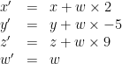
Clever! Now we can express the translate as a 4×4 matrix:

This is why all vectors in OpenGL are actually 4D, and all matrices in OpenGL are actually 4×4.

The orthographic projection matrix

If we assume that all of the vertices are transformed into Eye Coordinates by the model-view matrix, what does the scene look like if we just render it without setting the projection matrix (i.e., if we leave the projection matrix in its default identity state, so it doesn’t affect the vertices at all)? We will render everything in the cube from (-1, -1, -1) to (1, 1, 1). Recall that the Viewport transformation transforms the (x, y) coordinates into screen space such that (-1, -1) is in the lower-left and (1, 1) is in the upper right, and OpenGL clips any vertex with a z coordinate that is not in between -1 and 1. The geometry will be rendered without perspective — objects will appear to be the same size no matter how close they are, and the z coordinate will only be used for depth buffer tests and clipping.

This is an orthographic projection and it isn’t normally used for 3D graphics because it produces unrealistic images. However, it is frequently used in CAD tools and other diagrams, often in the form of an isometric projection. Such a projection is also ideal for drawing 2D graphics with OpenGL — for example when drawing the user interface on top of a 3D game, you will want to switch into an orthographic projection and turn off the depth buffer.

There is also a weirdness because OpenGL is supposed to use a right-handed coordinate system: the Z axis is inverted (recall that the -Z axis points away from the camera, but in the depth buffer, smaller z values are considered closer). To fix this, we can invert the Z coordinate by setting the GL_PROJECTION matrix to the following:

Now objects with smaller z coordinates will appear behind objects with larger z coordinates. That’s the basic principle of the orthographic projection matrix, but we can customise it by modifying the cube that defines our screen and clipping space. The glOrtho function modifies the projection matrix to an orthographic projection with a custom cube: its arguments are left, right, bottom, top, nearVal, farVal. To make things extra confusing, the nearVal and farVal are inverse Z coordinates; for example, nearVal = 3 and farVal = 5 implies that the Z clipping is between -3 and -5. I think this negative Z axis thing was a really bad idea.

Some simple calculations show that in order to linearly map the range [left, right] on to [-1, 1], the range [bottom, top] on to [-1, 1], and the range [-nearVal, –farVal] on to [-1, 1], we use the formula:

Using the same trick as with the translation matrix (assuming that w is always 1), we can express this with the orthographic projection matrix:

Which is precisely the matrix produced by glOrtho.

The perspective projection matrix

At last, we come to the perspective projection matrix, the projection matrix used for realistic 3D displays. The perspective projection is realistic because it causes objects further in the distance to appear smaller. Like the orthographic projection, perspective is clipped (you need to specify near and far z coordinates, and any geometry outside of that range will not be drawn). However, the screen and clipping space is not a cube, but a square frustum (a square-based pyramid with the apex cut off). Indeed, if we set the near clipping plane to 0, the screen clipping region is a square-based pyramid with the camera as the apex (but we usually need a positive near clipping plane for the depth buffer to work).

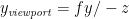
The gluPerspective function is used to set up the perspective projection matrix, and in this section, we analyse the maths behind the matrix it creates. It takes four parameters:

• fovy (“field-of-view y“): the vertical viewing angle. This is the angle, in degrees, from the top of the screen to the bottom.
• aspect: The aspect ratio, which controls the horizontal viewing angle relative to the vertical. For a non-stretched perspective, aspect should be the ratio of the screen width to height. For example, on a 640×480 display, aspect should be 4/3.
• zNear: The inverted z coordinate of the near clipping plane.
• zFar: The inverted z coordinate of the far clipping plane.

By the way, you can derive the fovx (“field-of-view x”) from aspect and fovy using trigonometry:

[Edit: Added the above paragraph after reader Bobby Bobson pointed out that my previous calculation for fovx was incorrect.]

As with glOrtho, the near and far clipping planes are inverted: zNear and zFar are always positive, even though z coordinates of objects in front of the camera are negative.

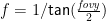
Let’s work out exactly how to go from 3D Eye Coordinates (again, assuming a fourth vector coordinate w which is always 1) to 2D screen coordinates with a depth buffer zvalue, in a perspective projection. First, we compute the 2D screen coordinates. The following diagram shows a side view of the scene in Eye Coordinate space. The camera frustum is pictured, bounded by the angle fovy and the Z clipping planes -zNear and -zFar. A blue triangle is visualised, representing a point at coordinate (y, z), where z is some arbitrary depth, and y lies on the edge of the frustum at that depth. Keep in mind that z must be a negative value.

Side view of the camera frustum

Simple trigonometry tells us the relationship between y, z and fovy: in the blue right-angled triangle, y is the opposite edge, –z is the adjacent edge, and fovy/2 is the angle. Therefore, if we know z and fovy, we can compute y:

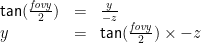
We can simplify the following maths if we define:

then:

At depth z, a Y eye coordinate value of y should map on to the viewport coordinate y = 1, as it is at the very top of the screen. Similarly, a Y eye coordinate value of –y should map onto viewport coordinate y = -1, and all intermediate Y values should map linearly across that range (because perspective projection is linear for all values at the same depth). That means for any (y, z) eye coordinate, we can divide by to compute the corresponding viewport coordinate. Thus, for any (y, z) eye coordinate, we can compute the corresponding viewport coordinate:

In the X axis, we find that at depth z, if y is the Y eye coordinate on the top edge of the frustum, the corresponding X eye coordinate on the right edge of the frustum is y × aspect. Therefore, using the same logic as above, for any (x, z) eye coordinate, we can compute the corresponding x viewport coordinate:

Finally, we need to move the z coordinate into the depth buffer space, such that –zNear maps onto -1, –zFar maps onto 1, and all Z eye coordinates in between are moved into the range [-1, 1]. We could map onto this space any way we like (linear might be a simple and obvious choice), but we don’t actually want a linear mapping: that would imply that all Z coordinates in that range have equal importance. We actually want to give coordinates close to the camera a much larger portion of the depth buffer than coordinates far from the camera. That is because near objects will be held to close scrutiny by the viewer, and thus need to be represented with fine detail in the depth buffer, whereas with far objects, it does not matter so much if they overlap. A good function is the reciprocal function, of the form .

The general form of this function is:

To satisfy our constraints on zNear and zFar, we obtain the equations:

We solve for m and c:

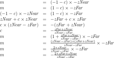
Hence, we have the equation:

The following chart gives an idea of how the perspective projection maps Z eye coordinate values onto depth buffer values, with zNear = 1 and zFar = 5:

Mapping Z eye coordinate values onto the depth buffer

Notice how the mapping is heavily skewed to favour objects near the front of the screen. Half of the depth buffer space is given to objects in the front 16% of the frustum space.

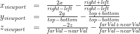
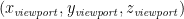
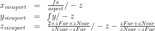
So our equations for transforming from eye coordinates (x, y, z) to viewport coordinates are:

But there’s a problem: Mathematically, these equations work fine, but they are non-linear transformations — all three involve division by z — so they cannot be represented by a matrix (recall that matrices represent functions that sum a constant multiple of each coordinate). So we have to cheat a little bit in order to use a matrix: we notice that the division by –z is consistent in all three equations, so we factor it out:

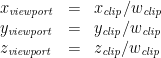
Note that by factoring out the division, the third equation gained a multiplication by z. If we ignore the “/ –z” part of each equation, we see that it is now a linear equation suitable for encoding as a matrix. Thus, we invent “Clip Coordinates” — basically the above equations with the –z factored out. Rather than setting w to 1 as usual, we set it to –z, for reasons that will soon become clear:

We can now redefine the viewport coordinates in terms of the clip coordinates, using the fact that the w clip coordinate has been set to –z:

The beauty of separating these two steps is that the first step can now be achieved with a matrix, while the second step is extremely simple. In OpenGL, the projection matrix (GL_PROJECTION) transforms Eye Coordinates to Clip Coordinates (not Viewport Coordinates). We can rewrite the above eye-to-clip equations as a matrix (assuming that the w eye coordinate is always 1):

That is, indeed, the projection matrix created by gluPerspective. Because we can’t express the clip-to-viewport transformation as a matrix, OpenGL does it for us, probably using specialised hardware to make it extremely efficient. So in the end, we can achieve the perspective transformation using a matrix and an extra bit of specialised code, and the whole thing is really really fast.

One final point: As I said earlier, the newer versions of OpenGL (version 3.0, or ES 2.0) don’t have any built-in matrix support. There is no GL_MODELVIEW or GL_PROJECTION matrix. These OpenGL versions require that you write shaders to do all of this work yourself (the shaders run on the GPU). But the principle is the same: you would create a projection matrix just like the one above, and multiply it by each vertex in the vertex shader. The output of the vertex shader is clip coordinates (not viewport coordinates) — OpenGL still performs the “divide by w” step automatically.

Edited 2017-03-25: Updated broken links to the new Khronos website.
Edited 2017-03-25: Fixed fovx calculation.